Get started with limpca.
Benaiche Nadia, Sébastien Franceschini, Martin Manon, Thiel Michel, Govaerts Bernadette
May 28, 2024
Source:vignettes/limpca.Rmd
limpca.RmdIntroduction
About the package
This package was created to analyse models with high-dimensional data
and a multi-factor design of experiment. limpca stands for
linear modeling of high-dimensional
designed data based on the ASCA (ANOVA-Simultaneous Component Analysis)
and APCA (ANOVA-Principal Component Analysis) family of
methods. These methods combine ANOVA with a General Linear Model (GLM)
decomposition and PCA. They provide powerful visualization tools for
multivariate structures in the space of each effect of the statistical
model linked to the experimental design. Details on the methods used and
the package implementation can be found in the articles of Thiel, Féraud, and Govaerts (2017), Guisset, Martin, and Govaerts (2019) and Thiel et al. (2023).
Therefore, ASCA/APCA are highly informative modeling and
visualisation tools to analyse -omics data tables in a multivariate
framework and act as a complement to differential expression analyses
methods such as limma (Ritchie et
al. (2015)).
Vignettes description
Get started with limpca(this vignette): This vignette is a short application oflimpcaon theUCHdataset with data visualisation, exploration (PCA), GLM decomposition and ASCA modelling. The ASCA model used in this example is a three-way ANOVA with fixed effects.Analysis of the UCH dataset with limpca: This vignette is an extensive application of
limpcaon theUCHdataset with data visualisation, exploration (PCA), GLM decomposition and ASCA/APCA/ASCA-E modelling. The applied model is a three-way ANOVA with fixed effects. This document presents all the usual steps of the analysis, from importing the data to visualising the results.Analysis of the Trout dataset with limpca: This vignette is an extensive application of
limpcaon theTroutdataset with data visualisation, exploration (PCA), GLM decomposition and ASCA/APCA/ASCA-E modelling. The applied model involves three main effects and their two-way interaction terms. It also compares the results of ASCA to a univariate ANOVA modeling.
Installation and loading of the limpca package
limpca can be installed from Bioconductor:
if (!requireNamespace("BiocManager", quietly = TRUE))
    install.packages("BiocManager")

BiocManager::install("limpca")
And then loaded into your R session:
For any enquiry, you can send an email to the package authors: bernadette.govaerts@uclouvain.be ; michel.thiel@uclouvain.be or manon.martin@uclouvain.be
Short application on the UCH dataset
Data object
In order to use the limpca core functions, the data need to be
formatted as a list (informally called an lmpDataList) with the
following elements: outcomes (multivariate matrix),
design (data.frame) and formula (character
string). The UCH data set is already formatted
appropriately and can be loaded from limpca with the
data function.
data("UCH")
str(UCH)
#> List of 3
#>  $ design  :'data.frame':    34 obs. of  5 variables:
#>   ..$ Hippurate: Factor w/ 3 levels "0","1","2": 1 1 1 1 1 1 2 2 2 2 ...
#>   ..$ Citrate  : Factor w/ 3 levels "0","2","4": 1 1 2 2 3 3 1 1 2 2 ...
#>   ..$ Dilution : Factor w/ 1 level "diluted": 1 1 1 1 1 1 1 1 1 1 ...
#>   ..$ Day      : Factor w/ 2 levels "2","3": 1 1 1 1 1 1 1 1 1 1 ...
#>   ..$ Time     : Factor w/ 2 levels "1","2": 1 2 1 2 1 2 1 2 1 2 ...
#>  $ outcomes: num [1:34, 1:600] 0.0312 0.0581 0.027 0.0341 0.0406 ...
#>   ..- attr(*, "dimnames")=List of 2
#>   .. ..$   : chr [1:34] "M2C00D2R1" "M2C00D2R2" "M2C02D2R1" "M2C02D2R2" ...
#>   .. ..$ X1: chr [1:600] "9.9917004" "9.9753204" "9.9590624" "9.9427436" ...
#>  $ formula : chr "outcomes ~ Hippurate + Citrate + Time + Hippurate:Citrate + Time:Hippurate + Time:Citrate + Hippurate:Citrate:Time"
Alternatively, the lmpDataList can be created with the function
data2LmpDataList :
- from scratch:
UCH2 <- data2LmpDataList(
   outcomes = UCH$outcomes,
   design = UCH$design,
   formula = UCH$formula
 )
#> | dim outcomes: 34x600
#> | formula: ~ Hippurate + Citrate + Time + Hippurate:Citrate + Time:Hippurate + Time:Citrate + Hippurate:Citrate:Time
#> | design variables (5):
#> * Hippurate (factor)
#> * Citrate (factor)
#> * Dilution (factor)
#> * Day (factor)
#> * Time (factor)- or from a
SummarizedExperiment:
se <- SummarizedExperiment(
   assays = list(
     counts = t(UCH$outcomes)), colData = UCH$design,
   metadata = list(formula = UCH$formula)
 )

UCH3 <- data2LmpDataList(se, assay_name = "counts")
#> | dim outcomes: 34x600
#> | formula: ~ Hippurate + Citrate + Time + Hippurate:Citrate + Time:Hippurate + Time:Citrate + Hippurate:Citrate:Time
#> | design variables (5):
#> * Hippurate (factor)
#> * Citrate (factor)
#> * Dilution (factor)
#> * Day (factor)
#> * Time (factor)
SummarizedExperiment is a generic data container that
stores rectangular matrices of experimental results. See Morgan et al. (2023) for more information.
Data visualisation
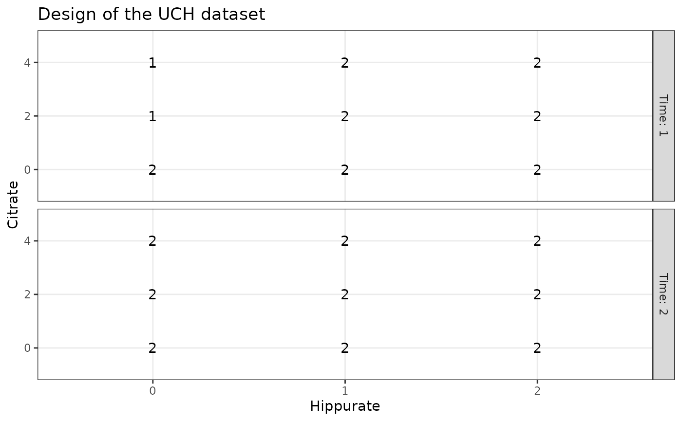
The design can be visualised with plotDesign().
# design
plotDesign(
    design = UCH$design, x = "Hippurate",
    y = "Citrate", rows = "Time",
    title = "Design of the UCH dataset"
)
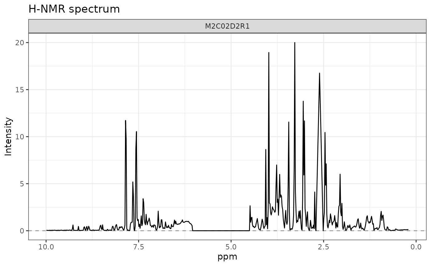
# row 3 of outcomes
plotLine(
    Y = UCH$outcomes,
    title = "H-NMR spectrum",
    rows = c(3),
    xlab = "ppm",
    ylab = "Intensity"
)
PCA
ResPCA <- pcaBySvd(UCH$outcomes)
pcaScreePlot(ResPCA, nPC = 6)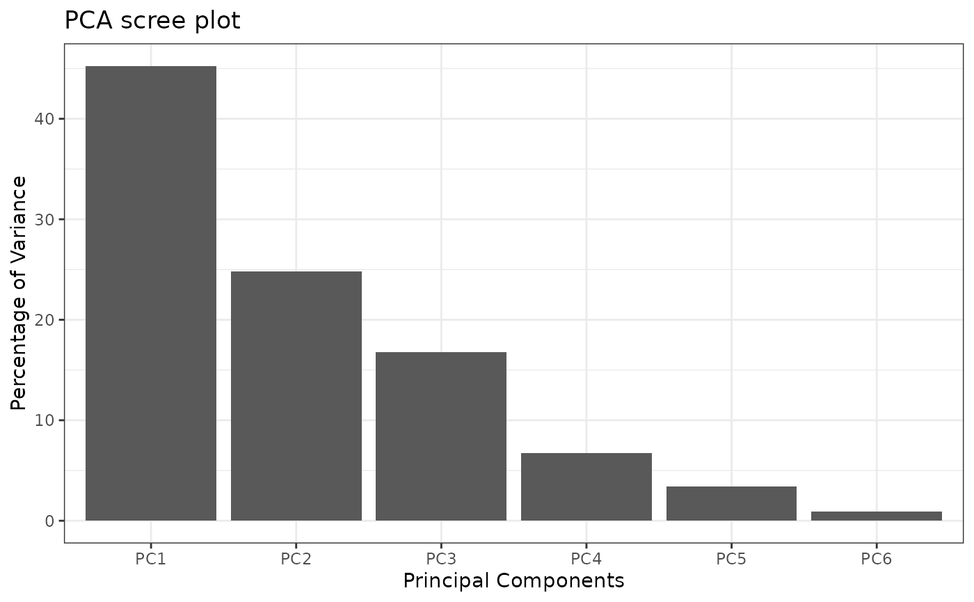
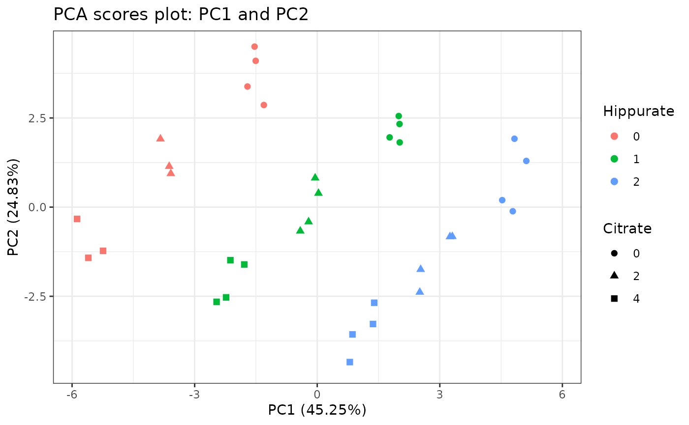
pcaScorePlot(
    resPcaBySvd = ResPCA, axes = c(1, 2),
    title = "PCA scores plot: PC1 and PC2",
    design = UCH$design,
    color = "Hippurate", shape = "Citrate",
    points_labs_rn = FALSE
)
Model estimation and effect matrix decomposition
# Model matrix generation
resMM <- lmpModelMatrix(UCH)

# Model estimation and effect matrices decomposition
resEM <- lmpEffectMatrices(resMM)
Effect matrix test of significance and importance measure
# Effects importance
resEM$varPercentagesPlot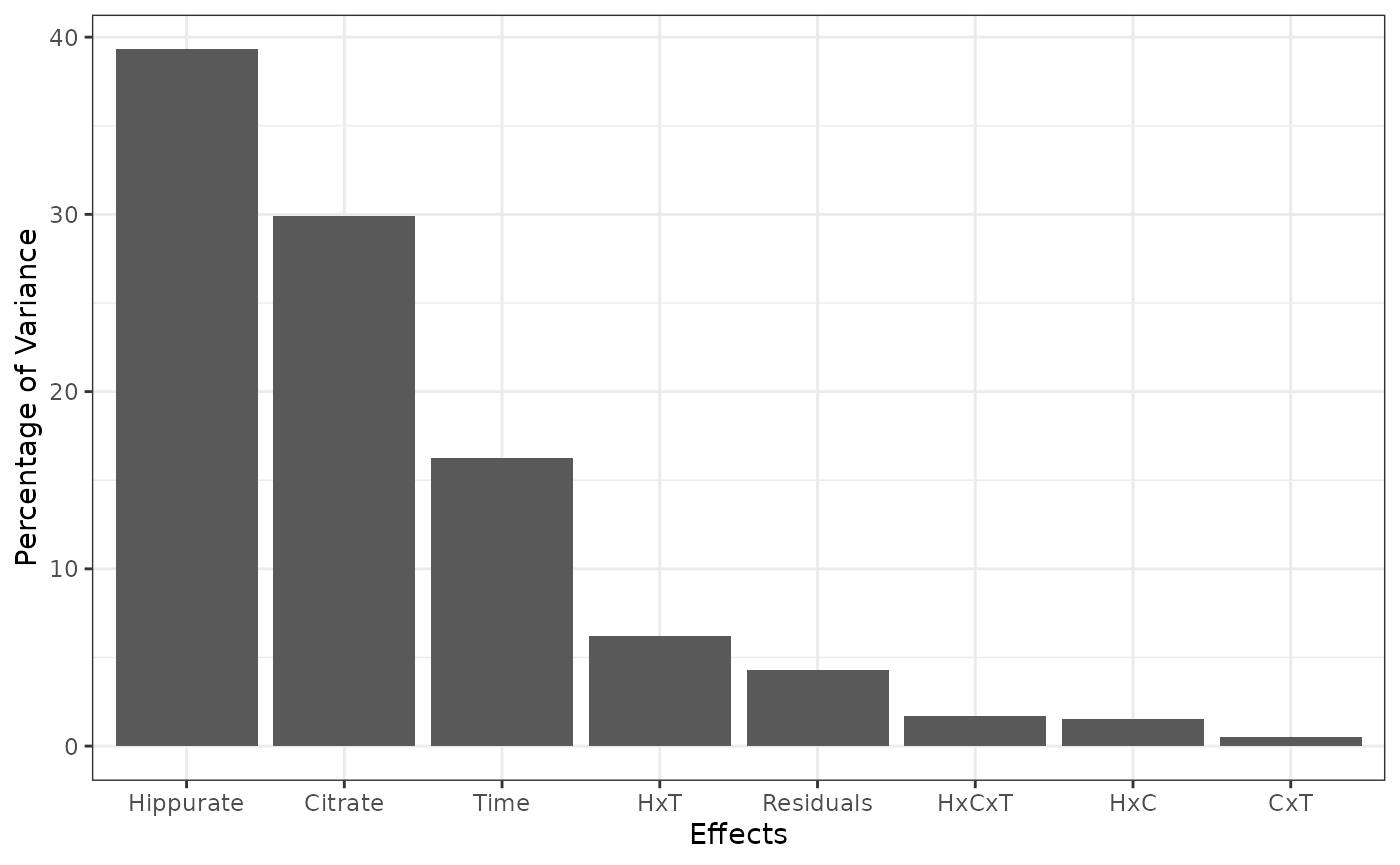
# Bootstrap tests
resBT <- lmpBootstrapTests(resLmpEffectMatrices = resEM, nboot = 100)
resBT$resultsTable
#>                        % of variance (T III) Bootstrap p-values
#> Hippurate                              39.31             < 0.01
#> Citrate                                29.91             < 0.01
#> Time                                   16.24             < 0.01
#> Hippurate:Citrate                       1.54               0.12
#> Hippurate:Time                          6.23             < 0.01
#> Citrate:Time                            0.54               0.42
#> Hippurate:Citrate:Time                  1.68               0.08
#> Residuals                               4.30                  -
ASCA decomposition
# ASCA decomposition
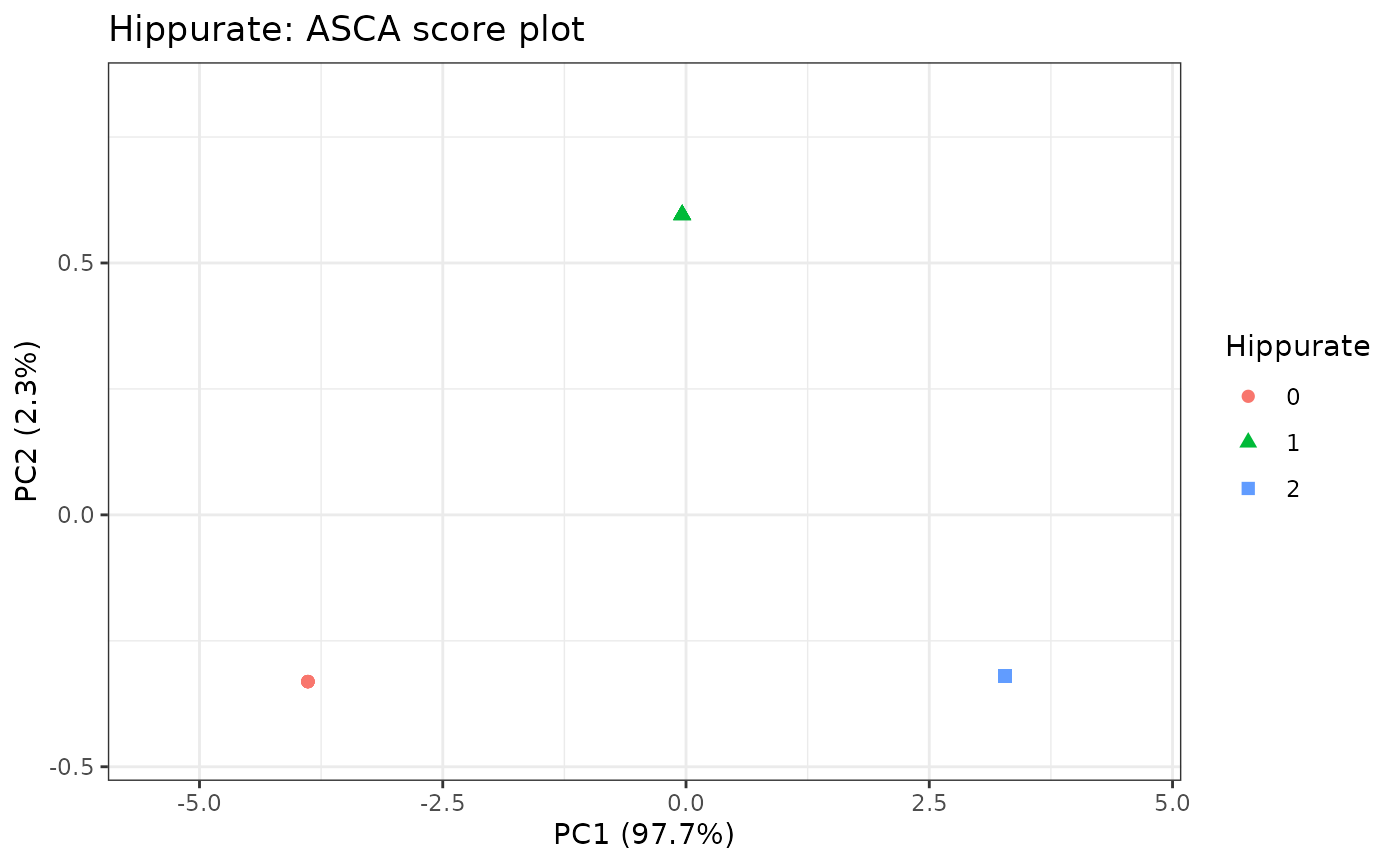
resASCA <- lmpPcaEffects(resLmpEffectMatrices = resEM, method = "ASCA")

# Scores Plot for the hippurate
lmpScorePlot(resASCA,
    effectNames = "Hippurate",
    color = "Hippurate", shape = "Hippurate"
)
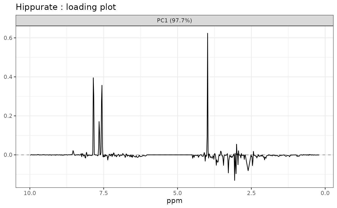
# Loadings Plot for the hippurate
lmpLoading1dPlot(resASCA,
    effectNames = c("Hippurate"),
    axes = 1, xlab = "ppm"
)
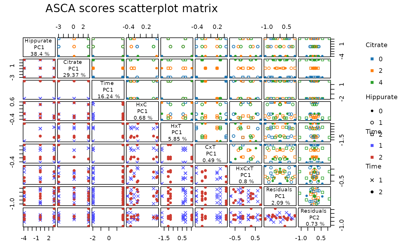
# Scores ScatterPlot matrix
lmpScoreScatterPlotM(resASCA,
    PCdim = c(1, 1, 1, 1, 1, 1, 1, 2),
    modelAbbrev = TRUE,
    varname.colorup = "Citrate",
    varname.colordown = "Time",
    varname.pchup = "Hippurate",
    varname.pchdown = "Time",
    title = "ASCA scores scatterplot matrix"
)
sessionInfo
sessionInfo()
#> R version 4.4.0 (2024-04-24)
#> Platform: x86_64-pc-linux-gnu
#> Running under: Ubuntu 22.04.4 LTS
#>
#> Matrix products: default
#> BLAS:   /usr/lib/x86_64-linux-gnu/openblas-pthread/libblas.so.3
#> LAPACK: /usr/lib/x86_64-linux-gnu/openblas-pthread/libopenblasp-r0.3.20.so;  LAPACK version 3.10.0
#>
#> locale:
#>  [1] LC_CTYPE=C.UTF-8       LC_NUMERIC=C           LC_TIME=C.UTF-8
#>  [4] LC_COLLATE=C.UTF-8     LC_MONETARY=C.UTF-8    LC_MESSAGES=C.UTF-8
#>  [7] LC_PAPER=C.UTF-8       LC_NAME=C              LC_ADDRESS=C
#> [10] LC_TELEPHONE=C         LC_MEASUREMENT=C.UTF-8 LC_IDENTIFICATION=C
#>
#> time zone: UTC
#> tzcode source: system (glibc)
#>
#> attached base packages:
#> [1] stats4    stats     graphics  grDevices utils     datasets  methods
#> [8] base
#>
#> other attached packages:
#>  [1] SummarizedExperiment_1.34.0 Biobase_2.64.0
#>  [3] GenomicRanges_1.56.0        GenomeInfoDb_1.40.1
#>  [5] IRanges_2.38.0              S4Vectors_0.42.0
#>  [7] BiocGenerics_0.50.0         MatrixGenerics_1.16.0
#>  [9] matrixStats_1.3.0           limpca_1.1.0
#> [11] BiocStyle_2.32.0
#>
#> loaded via a namespace (and not attached):
#>  [1] gtable_0.3.5            xfun_0.44               bslib_0.7.0
#>  [4] ggplot2_3.5.1           ggrepel_0.9.5           lattice_0.22-6
#>  [7] vctrs_0.6.5             tools_4.4.0             generics_0.1.3
#> [10] parallel_4.4.0          tibble_3.2.1            fansi_1.0.6
#> [13] highr_0.11              pkgconfig_2.0.3         Matrix_1.7-0
#> [16] tidyverse_2.0.0         desc_1.4.3              lifecycle_1.0.4
#> [19] GenomeInfoDbData_1.2.12 farver_2.1.2            stringr_1.5.1
#> [22] compiler_4.4.0          textshaping_0.4.0       munsell_0.5.1
#> [25] ggsci_3.1.0             codetools_0.2-20        htmltools_0.5.8.1
#> [28] sass_0.4.9              yaml_2.3.8              tidyr_1.3.1
#> [31] pkgdown_2.0.9           pillar_1.9.0            crayon_1.5.2
#> [34] jquerylib_0.1.4         DelayedArray_0.30.1     cachem_1.1.0
#> [37] iterators_1.0.14        abind_1.4-5             foreach_1.5.2
#> [40] tidyselect_1.2.1        digest_0.6.35           stringi_1.8.4
#> [43] reshape2_1.4.4          dplyr_1.1.4             purrr_1.0.2
#> [46] bookdown_0.39           labeling_0.4.3          fastmap_1.2.0
#> [49] grid_4.4.0              colorspace_2.1-0        cli_3.6.2
#> [52] SparseArray_1.4.8       magrittr_2.0.3          S4Arrays_1.4.1
#> [55] utf8_1.2.4              withr_3.0.0             scales_1.3.0
#> [58] UCSC.utils_1.0.0        rmarkdown_2.27          XVector_0.44.0
#> [61] httr_1.4.7              ragg_1.3.2              memoise_2.0.1
#> [64] evaluate_0.23           knitr_1.46              doParallel_1.0.17
#> [67] rlang_1.1.3             Rcpp_1.0.12             glue_1.7.0
#> [70] BiocManager_1.30.23     jsonlite_1.8.8          plyr_1.8.9
#> [73] R6_2.5.1                systemfonts_1.1.0       fs_1.6.4
#> [76] zlibbioc_1.50.0